Getting started
This page only provides an initial guide that illustrates the SEM workflow using the Python API. For a more comprehensive overview of how things work under the hood, refer to the Detailed Functionality page. If you are interested in using SEM from the command line, check out the Command Line Interface page instead.
SEM operates on simulation campaigns, which consist in a collection of results obtained from running a specific ns-3 simulation script with possibly varying command line parameters.
Simulation campaigns are saved in a single folder for portability, and are accessible through a CampaignManager object. Through this class it’s possible to create new campaigns, load existing ones, run simulations and export results to a variety of formats for analysis and plotting.
In the following sections we will use SEM to go from a vanilla ns-3 installation (assumed to be available at ./examples/ns-3) to plots visualizing the results, in as few commands as possible. A script containing many commands of this section is available at the sem project github, under examples/wifi_example.py.
Creating and loading a simulation campaign
Creation of a new campaign requires:
- The path of the ns-3 installation to use
- The name of the simulation script that will be run
- The location of the folder where the campaign will be saved.
We can create a campaign using the following instructions in a Python interpreter or script:
>>> import sem
>>> ns_path = 'examples/ns-3'
>>> script = 'wifi-multi-tos'
>>> campaign_dir = '/tmp/wifi-plotting-example'
>>> campaign = sem.CampaignManager.new(ns_path, script, campaign_dir, overwrite=True)
Internally, SEM also checks whether the path points to a valid ns-3 installation, and whether the script is actually available for execution or not. If a simulation campaign already exists at the specified campaign_dir, and if it points to the same ns_path and script values, that campaign is loaded instead. Otherwise, the campaign_dir folder is created from scratch and a new campaign is created.
CampaignManager objects can also be directly printed to inspect the status of the campaign:
>>> print(campaign)
--- Campaign info ---
script: wifi-multi-tos
params: ['nWifi', 'distance', 'simulationTime', 'useRts', 'mcs',
         'channelWidth', 'useShortGuardInterval']
HEAD: 9386dc7d106fd9241ff151195a0e6e5cb954d363
---------------------
Note that, additionally to the path and script we specified in the campaign creation process, SEM also retrieved a list of the available script parameters and the SHA of the current HEAD of the git repository at the ns-3 path.
Running simulations
Simulations can be run by specifying a list of parameter combinations.
>>> param_combination = {
...    'nWifi': 1,
...    'distance': 1,
...    'simulationTime': 10,
...    'useRts': False,
...    'mcs': 7,
...    'channelWidth': 20,
...    'useShortGuardInterval': False,
...    'RngRun': 0
... }
>>> campaign.run_simulations([param_combination])

Running simulations: 100% 1/1 [00:10<00:00, 10.81s/simulation]
As simulations are run, the results are also saved in the campaign database, at the previously specified campaign_dir path. After the simulation finishes, the results (i.e., any generated output files and the standard output) are added to the database and can be retrieved later on. A progress bar is displayed to indicate progress and give an estimate of the remaining time.
Multiple simulations corresponding to the exploration of a parameter space can be easily run by employing the list_param_combinations function, which can take a dictionary specifying multiple values for a key and translate it into a list of dictionaries specifying all combinations of parameter values. For example, let’s try the same simulation parameters as before, but perform the simulations both for the true and false values of the useRts parameter:
>>> param_combinations = {
...     'nWifi': 1,
...     'distance': 1,
...     'simulationTime': 10,
...     'useRts': [False, True],
...     'mcs': 7,
...     'channelWidth': 20,
...     'useShortGuardInterval': False
... }
>>> campaign.run_missing_simulations(param_combinations,
...                                  runs=1)

Running simulations: 100% 1/1 [00:09<00:00,  9.63s/simulation]
From the output, it can be noticed that only one simulation was run: in fact, since we used the run_missing_simulations function, before running the specified simulations, SEM checked whether some results were already available in the database, found the previously executed simulation, and only performed the simulation for which no result employing the requested parameter combination was already available. Additionally, the run_missing_simulations function requires a runs parameter, specifying how many runs should be performed for each parameter combination. Note the difference with run_simulations: run_simulations will run all the simulations in the specified list, regardless of the number of already available reproductions we have. run_missing_simulations, instead, will only run the simulations that are needed to obtain runs repetitions of a set parameter combination (hence the need for the runs parameter, which is not required by run_simulations).
Finally, let’s make SEM run multiple simulations so that we have something to plot. In order to do this, first we define a new param_combinations dictionary, ranging the mcs parameter from 0 to 7 and turning on and off the RequestToSend and ShortGuardInterval parameters:
>>> param_combinations = {
...     'nWifi': 1,
...     'distance': 1,
...     'simulationTime': 10,
...     'useRts': [False, True],
...     'mcs': list(range(1, 8, 2)),
...     'channelWidth': 20,
...     'useShortGuardInterval': [False, True]
... }
>>> campaign.run_missing_simulations(param_combinations,
...                                  runs=2)

Running simulations: 100% 32/32 [02:57<00:00,  3.86s/simulation]
Exporting results
Results can be exported to the numpy and xarray formats for Python elaboration, and to a directory tree, .mat and .npy file formats for processing outside Python.
Available results can be inspected using the DatabaseManager object associated to the CampaignManager, and available as the db attribute of the campaign. For instance, let’s check out the first result:
>>> len(campaign.db.get_results())
32
>>> campaign.db.get_results()[0]
{
  'nWifi': 1,
  'distance': 1,
  'simulationTime': 10,
  'useRts': False,
  'mcs': 7,
  'channelWidth': 20,
  'useShortGuardInterval': False,
  'RngRun': 1,
  'id': '771e0511-43b9-4e33-aa6a-dc4266be24f1',
  'elapsed_time': 4.270819187164307,
  'stdout': 'Aggregated throughput: 49.2696 Mbit/s\n'
}
Results are returned as dictionaries, with a key-value pair for each available script parameter, and the following additional fields:
- RngRun: the –RngRun value that was used for this simulation (used to set the “seed” of the simulator’s random number generator);
- id: an unique identifier for the simulation;
- elapsed_time: the required time, in seconds, to run the simulation;
- stdout: the output of the simulation script.
At its current state, the SEM library supports automatic parsing of the stdout result field: in the following lines we will define a get_average_throughput function, which transforms strings formatted like the stdout field of the result above into float numbers containing the average throughput measured by the simulation. SEM will then use the function to automatically clean up the results before putting them in an xarray structure:
>>> def get_average_throughput(result):
...     # This function takes a result and parses its standard output to extract
...     # relevant information
...     return [float(result['output']['stdout'].split(" ")[-2])]

>>> results = campaign.get_results_as_xarray(param_combinations,
...                                          get_average_throughput,
...                                          ['AvgThroughput'], runs=2)

    <xarray.DataArray (useRts: 2, mcs: 8, useShortGuardInterval: 2, runs: 2)>
    array([[[[10.8351 , 10.8057 , 10.8163 ],
            [11.849  , 11.8549 , 11.7901 ]],

            [...]

            [[35.2868 , 35.3763 , 35.3044 ],
            [36.4903 , 36.4137 , 36.4432 ]]]])
    Coordinates:
      * useRts                 (useRts) <U5 'false' 'true'
      * mcs                    (mcs) int64 0 1 2 3 4 5 6 7
      * useShortGuardInterval  (useShortGuardInterval) <U5 'false' 'true'
      * runs                   (runs) int64 0 1 2
Finally, we can easily plot the obtained results by appropriately slicing the DataArray:
>>> import matplotlib
>>> matplotlib.use('Agg')
>>> import matplotlib.pyplot as plt
>>> import numpy as np
>>> # Iterate over all possible parameter values
>>> for useShortGuardInterval in [False, True]:
...   for useRts in [False, True]:
...       avg = results.sel(useShortGuardInterval=useShortGuardInterval,
...                         useRts=useRts).reduce(np.mean, 'runs')
...       std = results.sel(useShortGuardInterval=useShortGuardInterval,
...                         useRts=useRts).reduce(np.std, 'runs')
...       eb = plt.errorbar(x=param_combinations['mcs'], y=avg, yerr=6*std,
...                    label='SGI %s, RTS %s' % (useShortGuardInterval, useRts))
...       xlb = plt.xlabel('MCS')
...       ylb = plt.ylabel('Throughput [Mbit/s]')
>>> legend = plt.legend(loc='best')
>>> plt.savefig('docs/throughput.png')
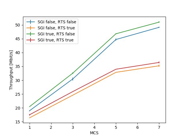
The plot obtained from the simulations.